Undiagnosed-1
Abstract
We took part in the Undiagnosed-1 SVAI Hackathon June 7-9, 2019. This was a collaborative, patient-focused genomics research case. Our goal was to combine the patient’s extensive genetic sequencing data and clinical notes with statistical machcine learning to produce a diagnosis. Our approach involved coarse-graining the patient data and computing a variety of correlation metrics with reference databases to produce a ranked list of potential diagnoses.
Data Preparation
The genetic sequencing data was provided in both raw reads (.bam files) and with genetic mutations identified by location (.vcf files). However, we wanted to correlate genetic mutations with potential diseases and so we first coarse-grained the genetic data by automatically annotating a reference genome with the .vcf files to produce a list of genes which had mutations (ie. a binary patient data vector).
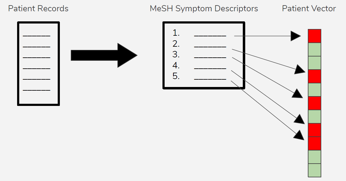
The patient’s clinical notes were provided as a series of scanned documents, which required us to read through everything provided and produce a summary table of symptoms, times, tests performed, treatments attempted, etc. We eventually standardized this data by converting all symptoms to MeSH terminology and produced a patient symptom data vector (again, a binary vector with 1 indicating symptom was present, 0 indicating symptom was absent).
We found several reference databases which mapped symptoms to disease, giving a larger score to symptoms which more strongly correlated with a given disease. We chose to use a database of generic diseases produced by scraping PubMed (Source) and another which focused on rare diseases (Source). Similarly, we found a database mapping genetic mutations to disease which we could use to compare to our patient data vector (Source).
Computation

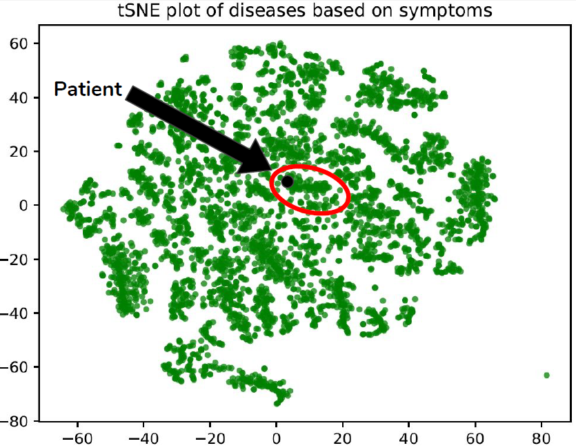
The most successful approach we found was to simply compute the projection of the patient data vector onto the reference database. This gave us a pseudo-correlation between patient symptoms or genetic mutations and diseases, which we could then sort to produce a ranked list of diagnoses. Another approach we took was to cluster the database of diseases and the unlabelled patient vector to see if the patient clustered with a related class of diseases. This approach was not easy to interpret but could be promising given more time to consider biases in the database itself.
The genetic database proved particularly difficult to use due to strong biases in the database. Given more time, we would have considered different methods of normalizing the scores in the database to minimize this effect.
Code
The following is a sample of the code we used. For the complete script, please see our GitHub repository.
First we define our databases. These are arrays with each row corresponding to a disease, each column corresponding to a symptom, and the element value indicating the correlation between the two.
symptoms = read_pickle(fname_symptom)
diseases = read_pickle(fname_disease)
symptom_disease_arr = read_pickle(fname_arr)
Next we set up our patient vector. These are the MeSH terms we collected from the patient’s documented medical history.
patient_symptoms_binary_vector = np.zeros((len(symptoms),))
patient_symptoms_manual = ['Body Weight', 'Psychophysiologic Disorders', 'Dyspepsia', 'Cachexia', 'Thinness', 'Polyuria',
                           'Vomiting', 'Nausea', 'Abdominal Pain', 'Fatigue', 'Constipation', 'Urinary Bladder, Overactive',
                           'Gastroparesis']
extra_patient_symptoms  = ['Weight Loss', 'Muscle Weakness', 'Urinary Incontinence', 'Muscle Spasticity', 'Muscular Atrophy',
                           'Neurologic Manifestations', 'Body Weight changes', 'Anorexia', 'Hyperkinesis', 'Vomiting, Anticipatory',
                           'Emaciation']

for i, symptom in enumerate(symptoms):
    if symptom in patient_symptoms_manual:
        patient_symptoms_binary_vector[i] = 1.0
We found that normalization was essential for reducing inherent bias int eh database.
B = np.array(symptom_disease_arr)

n_disease = B.shape[0]
n_symptom = B.shape[1]
assert B.shape[0] == 4219

row_sums = B.sum(axis=1)
B_norm = B / row_sums[:, numpy.newaxis]
row_sums = B_norm.sum(axis=1)
The simplest prediction was to compute the projection of the patient vector onto the database (ie. compute the correlation matrix) and rank the diseases by this ‘score’.
potential_diagnoses_1 = np.dot(B, patient_symptoms_binary_vector)
sorted_potential_diagnoses_1 = np.argsort(potential_diagnoses_1)[::-1]

print("Potential diagnoses from patient symptom vector")
for idx in range(10):
    print('Rank %d' % idx, diseases[sorted_potential_diagnoses_1[idx]], potential_diagnoses_1[sorted_potential_diagnoses_1[idx]])
Another approach was to perform unsupervised clustering via t-SNE to see which diseases the patient’s symptom vector clustered with. If the clusters are meaningful then the neighbouring points in the cluster would be most similar. We did not have enough time to refine this approach during the competition, but perhaps with some improvements we could get more meaningful clusters. Regardless, this is the code that we used:
def make_tsne_diagnosis(data, plot_fname, patient_vector, labels):
    # Add patient to data as an unlabelled 'disease'
    labels.append('Patient')
    data.append(patient_vector)

    # Perform PCA
    num_diseases = np.shape(data)[0]
    # Mean-center each feature
    feature_means = np.mean(data, axis=0)
    for disease_idx in range(num_diseases):
        data[disease_idx] = np.subtract(data[disease_idx], feature_means)
    # Get PCA-transformed data
    print("PCA Transformation")
    pca_vectors = PCA(n_components=50).fit(data)
    pca_transformed_data = pca_vectors.transform(data)

    # Perform tSNE
    tsne_embedded_symptoms = TSNE(n_components=2, verbose=1).fit_transform(pca_transformed_data)

    # Get distance from patient point to each disease
    distances = []
    for d in range(np.shape(tsne_embedded_symptoms)[0]-1):
        distances.append([labels[d], ((tsne_embedded_symptoms[d, 0]-tsne_embedded_symptoms[-1, 0])**2 + (tsne_embedded_symptoms[d, 1]-tsne_embedded_symptoms[-1, 1])**2)**0.5])

    # Rank diseases from nearest to farthest
    disease_rank = pd.DataFrame.from_records(distances, columns=['Disease', 'Distance'])
    print(disease_rank.sort_values('Distance', ascending=False))

    # Plot
    print("Plotting")
    plt.figure()
    plt.scatter(tsne_embedded_symptoms[:-1, 0], tsne_embedded_symptoms[:-1, 1], marker='.', color='green', alpha=0.75)
    plt.scatter(tsne_embedded_symptoms[-1, 0], tsne_embedded_symptoms[-1, 1], marker='.', color='black', alpha=1)
    plt.title("tSNE plot of diseases based on symptoms")
    plt.savefig(plot_fname)
    plt.show()
    # Save tSNE embedding
    with open(os.path.join(os.getcwd(), 'patient', 'patient_symptoms_v1_diagnosis.p'), 'wb') as f:
        pickle.dump(tsne_embedded_symptoms, f)
Overall, we learned a lot about handling incomplete data, coarse-graining for the sake of simplicity, and working under time pressure. It was a lot of fun, and we’re looking forward to our next hackathon!
